Act like a helpful tutor and exlain step-by-step solution with explanation and final answer:» Derive the thermodynamic basis for a three-dimensional cohesive zone model, starting from the first and second laws of
thermodynamics applied to a fracturing continuum, to establish the relation between the cohesive traction vector and the
displacement jump vector across a cohesive surface.
» Formulate the Helmholtz free energy per unit area of the cohesive surface as a function of an effective damage variable and a
non-damaging elastic part, consistent with the concept of damage mechanics in quasi-brittle materials.
» Deduce the constitutive law for the cohesive traction vector by taking the partial derivative of the formulated Helmholtz free
energy with respect to the components of the separation vector, ensuring it accounts for mixed-mode fracture conditions.
» Construct the evolution equation for the damage variable, incorporating a fracture energy-based criterion that governs the pro-
gressive degradation of the cohesive traction, and specify the loading-unloading conditions.
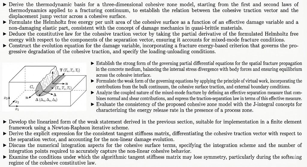
» Establish the strong form of the governing partial differential equations for the spatial fracture propagation
TET) in the concrete medium, balancing the internal stress divergence with body forces and ensuring equilibrium
across the cohesive interface.
: 4 » Formulate the weak form of the governing equations by applying the principle of virtual work, incorporating the
n
iG. £ TTT), contributions from the bulk continuum, the cohesive surface traction, and external boundary conditions.
/ aye » Analyze the coupled nature of the mixed-mode fracture by defining an effective separation measure that com-
ES BR Lie) bines normal and shear contributions, and express the traction-separation law in terms of this effective measure.
= » Evaluate the consistency of the proposed cohesive zone model with the J-integral concepts for
0 characterizing the energy release rate in the presence of a process zone.
» Develop the linearized form of the weak statement derived in the previous section, suitable for implementation in a finite element
framework using a Newton-Raphson iterative scheme.
» Derive the explicit expression for the consistent tangent stiffness matrix, differentiating the cohesive traction vector with respect to
the separation vector, and accounting for the non-linear damage evolution.
» Discuss the numerical integration aspects for the cohesive surface terms, specifying the integration scheme and the number of
integration points required to accurately capture the non-linear cohesive behavior.
» Examine the conditions under which the algorithmic tangent stiffness matrix may lose symmetry, particularly during the softening
regime of the cohesive constitutive law.
Question:
Act like a helpful tutor and exlain step-by-step solution with explanation and final answer:» Derive the thermodynamic basis for a three-dimensional cohesive zone model, starting from the first and second laws of
thermodynamics applied to a fracturing continuum, to establish the relation between the cohesive traction vector and the
displacement jump vector across a cohesive surface.
» Formulate the Helmholtz free energy per unit area of the cohesive surface as a function of an effective damage variable and a
non-damaging elastic part, consistent with the concept of damage mechanics in quasi-brittle materials.
» Deduce the constitutive law for the cohesive traction vector by taking the partial derivative of the formulated Helmholtz free
energy with respect to the components of the separation vector, ensuring it accounts for mixed-mode fracture conditions.
» Construct the evolution equation for the damage variable, incorporating a fracture energy-based criterion that governs the pro-
gressive degradation of the cohesive traction, and specify the loading-unloading conditions.
» Establish the strong form of the governing partial differential equations for the spatial fracture propagation
TET) in the concrete medium, balancing the internal stress divergence with body forces and ensuring equilibrium
across the cohesive interface.
: 4 » Formulate the weak form of the governing equations by applying the principle of virtual work, incorporating the
n
iG. £ TTT), contributions from the bulk continuum, the cohesive surface traction, and external boundary conditions.
/ aye » Analyze the coupled nature of the mixed-mode fracture by defining an effective separation measure that com-
ES BR Lie) bines normal and shear contributions, and express the traction-separation law in terms of this effective measure.
= » Evaluate the consistency of the proposed cohesive zone model with the J-integral concepts for
0 characterizing the energy release rate in the presence of a process zone.
» Develop the linearized form of the weak statement derived in the previous section, suitable for implementation in a finite element
framework using a Newton-Raphson iterative scheme.
» Derive the explicit expression for the consistent tangent stiffness matrix, differentiating the cohesive traction vector with respect to
the separation vector, and accounting for the non-linear damage evolution.
» Discuss the numerical integration aspects for the cohesive surface terms, specifying the integration scheme and the number of
integration points required to accurately capture the non-linear cohesive behavior.
» Examine the conditions under which the algorithmic tangent stiffness matrix may lose symmetry, particularly during the softening
regime of the cohesive constitutive law.
This is AI generated Response.
Asked by: Francis
Created at: 2026-02-25 08:03:32
Final Answer:
RenderedRaw Text
Did you like this answer?
Certainly! Let's walk through a **step-by-step solution** for the **development of a three-dimensional cohesive zone model** for quasi-brittle materials, as outlined in the provided text. I'll explain each step and provide the **final answer structure**.
---
## **Step 1: Thermodynamic Basis**
**Goal:**
Establish the relationship between the cohesive traction vector (**T**) and the displacement jump vector (**Δ**) across a cohesive surface using the first and second laws of thermodynamics.
**Explanation:**
- The first law (energy conservation) states that the internal energy change equals work done plus heat added.
- The second law (entropy production) requires that the process is thermodynamically admissible (irreversible processes must have non-negative dissipation).
- For a cohesive surface, **T** does work on the displacement jump **Δ**:
\[
\dot{\psi} = T \cdot \dot{\Delta} - D
\]
where \(\psi\) is the Helmholtz free energy per unit area, and \(D\) is the dissipation.
---
## **Step 2: Helmholtz Free Energy Formulation**
**Goal:**
Express the free energy per unit area (\(\psi\)) in terms of a damage variable (\(d\)) and separation (\(\Delta\)), allowing for both elastic and damage evolution.
**Explanation:**
- A typical form:
\[
\psi = (1 - d) \psi_{\text{elastic}}(\Delta)
\]
- \(d\) (: undamaged, 1: fully damaged)
- \(\psi_{\text{elastic}}(\Delta)\): elastic energy due to separation
---
## **Step 3: Constitutive Law for Cohesive Traction**
**Goal:**
Derive the expression for cohesive traction **T** as the derivative of free energy with respect to separation.
**Explanation:**
\[
T = \frac{\partial \psi}{\partial \Delta}
\]
- For mixed-mode conditions:
\[
T_i = (1 - d) \frac{\partial \psi_{\text{elastic}}}{\partial \Delta_i}
\]
where \(i\) represents the mode (normal, tangential, etc.)
---
## **Step 4: Evolution Equation for Damage Variable**
**Goal:**
Define how the damage variable \(d\) evolves with increasing separation, based on a fracture energy criterion.
**Explanation:**
- Damage growth should satisfy the energy dissipation condition.
- A common evolution equation:
\[
\dot{d} = f(\Delta, d)
\]
- Often, damage increases when the separation exceeds a threshold, linked to the fracture energy \(G_c\).
- Must specify loading/unloading rules (damage does not decrease on unloading).
---
## **Step 5: Strong and Weak Forms of Governing Equations**
**Goal:**
Formulate the governing equations for fracture propagation, ensuring equilibrium and compatibility across the interface.
**Explanation:**
- **Strong form:** Equilibrium equation with internal stress divergence + body forces = , and interface conditions involving cohesive traction.
- **Weak form:** Apply the principle of virtual work, integrating over the domain and cohesive surface.
---
## **Step 6: Mixed-Mode Fracture and Traction-Separation Law**
**Goal:**
Define an effective separation measure that combines normal and tangential modes, and express the traction-separation law accordingly.
**Explanation:**
- Effective separation:
\[
\Delta_{\text{eff}} = \sqrt{\left( \frac{\Delta_n}{\Delta_{n,c}} \right)^2 + \left( \frac{\Delta_s}{\Delta_{s,c}} \right)^2 }
\]
- \(\Delta_{n,c}, \Delta_{s,c}\): critical separations in each mode
- Traction law depends on \(\Delta_{\text{eff}}\).
---
## **Step 7: Linearization and Numerical Implementation**
**Goal:**
Linearize the weak form for use in finite element analysis and derive the consistent tangent stiffness matrix.
**Explanation:**
- Linearization yields the tangent matrix for Newton-Raphson iterations.
- The tangent is the derivative of **T** with respect to **Δ** (accounting for damage evolution).
---
## **Step 8: Numerical Integration and Accuracy**
**Goal:**
Ensure accurate computation of integrals over the cohesive surface, especially with nonlinear softening.
**Explanation:**
- Use appropriate quadrature schemes and sufficient integration points.
---
## **Step 9: Symmetry of Tangent Matrix**
**Goal:**
Check the symmetry of the stiffness matrix, noting that it may be lost in softening (damage) regimes.
**Explanation:**
- Symmetry relates to energy conservation—may not hold if damage evolution depends on direction/history.
---
# **Final Answer Summary**
**A three-dimensional cohesive zone model is developed by:**
1. **Deriving the thermodynamic relation** between cohesive traction and separation using the first and second laws.
2. **Formulating the Helmholtz free energy** as a function of separation and damage variable.
3. **Deducing the constitutive traction-separation law** via the energy derivative, accounting for mixed-mode effects.
4. **Constructing a damage evolution law** based on fracture energy criteria, detailing loading/unloading rules.
5. **Formulating the strong and weak forms** of the governing equations for implementation.
6. **Defining mixed-mode effective separation** and corresponding traction-separation laws.
7. **Linearizing the weak form** for finite element computation, deriving the tangent stiffness matrix.
8. **Ensuring accurate numerical integration** and discussing the potential loss of stiffness matrix symmetry during softening.
This comprehensive approach enables simulation of progressive fracture in quasi-brittle materials within a robust thermodynamic and computational framework.
Question:
humanise chesi simple ga evvu student raasinattu
This is AI generated Response.
Asked by: Francis
Created at: 2026-02-25 08:08:08
Final Answer:
RenderedRaw Text
Did you like this answer?
# Cohesive Zone Model for Quasi-Brittle Materials: A Simplified Explanation
## **Introduction**
This guide breaks down the development of a three-dimensional cohesive zone model used to study fractures in quasi-brittle materials. We'll go through each step clearly, focusing on the core concepts and processes involved.
---
## **Step 1: Thermodynamic Foundations**
### **Key Concepts**
- **First Law of Thermodynamics**: Energy cannot be created or destroyed.
- **Second Law of Thermodynamics**: Energy transformations increase entropy (disorder) in a system.
### **Application**
- We relate the cohesive traction vector (**T**) and displacement jump vector (**Δ**) using energy principles:
\[
\dot{\psi} = T \cdot \dot{\Delta} - D
\]
Here, \(D\) represents energy dissipation during the process.
---
## **Step 2: Helmholtz Free Energy**
### **What is it?**
The Helmholtz free energy (\(\psi\)) tells us about the energy available to do work at constant temperature and volume.
### **Formulation**
We express \(\psi\) as a function of a damage variable (\(d\)) and the displacement:
\[
\psi = (1 - d) \psi_{\text{elastic}}(\Delta)
\]
- \(d = 0\) means no damage; \(d = 1\) means total damage.
---
## **Step 3: Cohesive Traction Law**
### **Understanding Cohesive Traction**
Cohesive traction is the force per unit area acting across the cohesive surface.
### **Derivation**
To find **T**, we take the derivative of \(\psi\) with respect to **Δ**:
\[
T = \frac{\partial \psi}{\partial \Delta}
\]
For different fracture modes:
\[
T_i = (1 - d) \frac{\partial \psi_{\text{elastic}}}{\partial \Delta_i}
\]
---
## **Step 4: Damage Evolution Equation**
### **Purpose**
We need to describe how damage evolves as the material is loaded.
### **Formulation**
A common equation is:
\[
\dot{d} = f(\Delta, d)
\]
This indicates that damage increases when the separation exceeds a certain threshold, based on fracture energy.
---
## **Step 5: Governing Equations**
### **Strong Form**
This form includes the balance of forces:
- Internal stress divergence + body forces = 0.
### **Weak Form**
We apply the principle of virtual work, integrating over the domain and cohesive surface to account for all interactions.
---
## **Step 6: Mixed-Mode Fracture**
### **Effective Separation Measure**
To handle different types of fractures, we define an effective separation:
\[
\Delta_{\text{eff}} = \sqrt{\left( \frac{\Delta_n}{\Delta_{n,c}} \right)^2 + \left( \frac{\Delta_s}{\Delta_{s,c}} \right)^2 }
\]
### **Traction-Separation Relationship**
This relationship links the cohesive traction to the effective separation measure.
---
## **Step 7: Numerical Implementation**
### **Linearization**
To use the model in finite element analysis, we need to express the equations in a linearized form suitable for numerical methods.
### **Tangent Stiffness Matrix**
We derive this matrix by differentiating the traction with respect to separation, considering damage evolution.
---
## **Step 8: Numerical Integration**
### **Integration Accuracy**
We need to ensure accurate numerical integration of the cohesive behavior by choosing appropriate methods and enough integration points.
---
## **Step 9: Symmetry of Stiffness Matrix**
### **Loss of Symmetry**
The tangent stiffness matrix may lose symmetry during the softening phase of the material, particularly when damage evolves.
---
## **Final Summary**
This cohesive zone model provides a comprehensive framework for analyzing fractures in quasi-brittle materials. By understanding the thermodynamic principles, formulating energy relationships, and implementing numerical methods, we can effectively simulate and predict the behavior of materials under stress.
VIPSolutions focuses on clear, step‑by‑step explanations so you can learn quickly. Whether you need an AI‑generated walkthrough or a short hint to get unstuck, each solution is organized for fast reading and easy review later.
Search similar questions, compare approaches, and bookmark the best answers for revision. Our goal is simple: quick, reliable study help that feels natural—not noisy.
 » Derive the thermodynamic basis for a three-dimensional cohesive zone model, starting from the first and second laws of
thermodynamics applied to a fracturing continuum, to establish the relation between the cohesive traction vector and the
displacement jump vector across a cohesive surface.
» Formulate the Helmholtz free energy per unit area of the cohesive surface as a function of an effective damage variable and a
non-damaging elastic part, consistent with the concept of damage mechanics in quasi-brittle materials.
» Deduce the constitutive law for the cohesive traction vector by taking the partial derivative of the formulated Helmholtz free
energy with respect to the components of the separation vector, ensuring it accounts for mixed-mode fracture conditions.
» Construct the evolution equation for the damage variable, incorporating a fracture energy-based criterion that governs the pro-
gressive degradation of the cohesive traction, and specify the loading-unloading conditions.
» Establish the strong form of the governing partial differential equations for the spatial fracture propagation
TET) in the concrete medium, balancing the internal stress divergence with body forces and ensuring equilibrium
across the cohesive interface.
: 4 » Formulate the weak form of the governing equations by applying the principle of virtual work, incorporating the
n
iG. £ TTT), contributions from the bulk continuum, the cohesive surface traction, and external boundary conditions.
/ aye » Analyze the coupled nature of the mixed-mode fracture by defining an effective separation measure that com-
ES BR Lie) bines normal and shear contributions, and express the traction-separation law in terms of this effective measure.
= » Evaluate the consistency of the proposed cohesive zone model with the J-integral concepts for
0 characterizing the energy release rate in the presence of a process zone.
» Develop the linearized form of the weak statement derived in the previous section, suitable for implementation in a finite element
framework using a Newton-Raphson iterative scheme.
» Derive the explicit expression for the consistent tangent stiffness matrix, differentiating the cohesive traction vector with respect to
the separation vector, and accounting for the non-linear damage evolution.
» Discuss the numerical integration aspects for the cohesive surface terms, specifying the integration scheme and the number of
integration points required to accurately capture the non-linear cohesive behavior.
» Examine the conditions under which the algorithmic tangent stiffness matrix may lose symmetry, particularly during the softening
regime of the cohesive constitutive law.
» Derive the thermodynamic basis for a three-dimensional cohesive zone model, starting from the first and second laws of
thermodynamics applied to a fracturing continuum, to establish the relation between the cohesive traction vector and the
displacement jump vector across a cohesive surface.
» Formulate the Helmholtz free energy per unit area of the cohesive surface as a function of an effective damage variable and a
non-damaging elastic part, consistent with the concept of damage mechanics in quasi-brittle materials.
» Deduce the constitutive law for the cohesive traction vector by taking the partial derivative of the formulated Helmholtz free
energy with respect to the components of the separation vector, ensuring it accounts for mixed-mode fracture conditions.
» Construct the evolution equation for the damage variable, incorporating a fracture energy-based criterion that governs the pro-
gressive degradation of the cohesive traction, and specify the loading-unloading conditions.
» Establish the strong form of the governing partial differential equations for the spatial fracture propagation
TET) in the concrete medium, balancing the internal stress divergence with body forces and ensuring equilibrium
across the cohesive interface.
: 4 » Formulate the weak form of the governing equations by applying the principle of virtual work, incorporating the
n
iG. £ TTT), contributions from the bulk continuum, the cohesive surface traction, and external boundary conditions.
/ aye » Analyze the coupled nature of the mixed-mode fracture by defining an effective separation measure that com-
ES BR Lie) bines normal and shear contributions, and express the traction-separation law in terms of this effective measure.
= » Evaluate the consistency of the proposed cohesive zone model with the J-integral concepts for
0 characterizing the energy release rate in the presence of a process zone.
» Develop the linearized form of the weak statement derived in the previous section, suitable for implementation in a finite element
framework using a Newton-Raphson iterative scheme.
» Derive the explicit expression for the consistent tangent stiffness matrix, differentiating the cohesive traction vector with respect to
the separation vector, and accounting for the non-linear damage evolution.
» Discuss the numerical integration aspects for the cohesive surface terms, specifying the integration scheme and the number of
integration points required to accurately capture the non-linear cohesive behavior.
» Examine the conditions under which the algorithmic tangent stiffness matrix may lose symmetry, particularly during the softening
regime of the cohesive constitutive law.