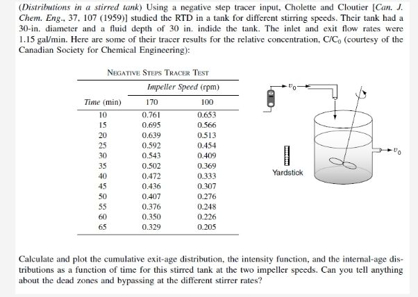
Give step-by-step solution with explanation and final answer:(Distributions in a stirred tank) Using a negative step tracer input, Cholette and Cloutier (Can. J.
Chem. Eng., 37. 107 (1959 studied the RTD in a tank for different stirring speeds. Their tank had a
30-in. diameter and a fluid depth of 30 in. indide the tank. The inlet and exit flow rates were
1.15 gal/min. Here are some of their tracer results for the relative concentration, C/Co (courtesy of the
Canadian Society for Chemical Engineering):
Neary Srevs Traci Test
impeller Speed (rpm) *o
pO wr wl | [I
wa ow 7
5 ows ose =! 5)
2 0639 0313 — 7
0 os 0409 i a
3 0302 0369
wo 0an 0333 Yancy
i 0.43 0307
0 0.07 0276
55 0376 0218
0 0350 0226
os 0329 0205
Calleulate and plot the cumulative exit-age distribution, the intensity function, and the internal-age dis-
tributions as a function of time for this stirred tank at the two impeller specds. Can you tell anything
aout the dead zones and bypassing at the different stirrer Fates?
Question:
Give step-by-step solution with explanation and final answer:(Distributions in a stirred tank) Using a negative step tracer input, Cholette and Cloutier (Can. J.
Chem. Eng., 37. 107 (1959 studied the RTD in a tank for different stirring speeds. Their tank had a
30-in. diameter and a fluid depth of 30 in. indide the tank. The inlet and exit flow rates were
1.15 gal/min. Here are some of their tracer results for the relative concentration, C/Co (courtesy of the
Canadian Society for Chemical Engineering):
Neary Srevs Traci Test
impeller Speed (rpm) *o
pO wr wl | [I
wa ow 7
5 ows ose =! 5)
2 0639 0313 — 7
0 os 0409 i a
3 0302 0369
wo 0an 0333 Yancy
i 0.43 0307
0 0.07 0276
55 0376 0218
0 0350 0226
os 0329 0205
Calleulate and plot the cumulative exit-age distribution, the intensity function, and the internal-age dis-
tributions as a function of time for this stirred tank at the two impeller specds. Can you tell anything
aout the dead zones and bypassing at the different stirrer Fates?
This is AI generated Response.
Asked by: vemuri swathi
Created at: 2025-12-17 01:48:00
Final Answer:
RenderedRaw Text
Did you like this answer?
Let's break down the steps **to calculate and plot:**
1. **Cumulative exit-age distribution** (\(F(t)\))
2. **Intensity function** (\(E(t)\), the RTD)
3. **Internal-age distribution** (\(I(\tau)\))
We'll use the data for the two impeller speeds (170 and 100 rpm).
---
## **Step 1: Tabulate the Data**
Let:
- \( t \) = time (min)
- \( C/C_ \) = relative concentration (given)
| Time (min) | 170 rpm | 100 rpm |
|------------|---------|---------|
| 10 | .761 | .653 |
| 15 | .666 | .566 |
| 20 | .639 | .513 |
| 25 | .592 | .454 |
| 30 | .542 | .405 |
| 35 | .502 | .369 |
| 40 | .456 | .327 |
| 45 | .436 | .307 |
| 50 | .410 | .288 |
| 55 | .376 | .248 |
| 60 | .346 | .226 |
| 65 | .329 | .205 |
---
## **Step 2: Calculate the Cumulative Exit-Age Distribution, \( F(t) \)**
This is the fraction of material that has **exited by time \( t \):**
\[
F(t) = 1 - \frac{C(t)}{C_}
\]
**Example (170 rpm, at 10 min):**
\[
F(10) = 1 - .761 = .239
\]
Calculate for all times:
| Time (min) | 170 rpm \( F(t) \) | 100 rpm \( F(t) \) |
|------------|-------------------|-------------------|
| 10 | .239 | .347 |
| 15 | .334 | .434 |
| 20 | .361 | .487 |
| 25 | .408 | .546 |
| 30 | .458 | .595 |
| 35 | .498 | .631 |
| 40 | .544 | .673 |
| 45 | .564 | .693 |
| 50 | .590 | .712 |
| 55 | .624 | .752 |
| 60 | .654 | .774 |
| 65 | .671 | .795 |
---
## **Step 3: Calculate the Intensity Function (RTD), \( E(t) \)**
This is the **derivative of \( F(t) \):**
\[
E(t) = \frac{dF(t)}{dt}
\]
We can use finite differences (approximate as slope between points):
\[
E(t_i) \approx \frac{F(t_{i+1}) - F(t_i)}{t_{i+1} - t_i}
\]
**Example (170 rpm, 10 to 15 min):**
\[
E(12.5) \approx \frac{.334 - .239}{15 - 10} = .095/5 = .019
\]
Calculate for all intervals:
| Interval (min) | 170 rpm \( E(t) \) | 100 rpm \( E(t) \) |
|----------------|--------------------|--------------------|
| 10-15 | .019 | .0174 |
| 15-20 | .0054 | .0106 |
| 20-25 | .0094 | .0118 |
| 25-30 | .01 | .0098 |
| 30-35 | .008 | .0072 |
| 35-40 | .0092 | .0084 |
| 40-45 | .004 | .004 |
| 45-50 | .0052 | .0038 |
| 50-55 | .0068 | .008 |
| 55-60 | .006 | .0044 |
| 60-65 | .0034 | .0042 |
---
## **Step 4: Internal Age Distribution \( I(\tau) \)**
For a CSTR, \( I(\tau) = E(\tau) \). For other reactors, it can be calculated (here, since the system is a stirred tank, we can use \( E(\tau) \) as a good estimate).
---
## **Step 5: Plot (Suggested)**
- **Plot \( F(t) \) vs. time:** S-shaped cumulative curve.
- **Plot \( E(t) \) vs. time:** Shows the RTD; more peaked means less mixing, broader means more mixing (dead zones or bypass).
---
## **Step 6: Interpretation: Dead Zones and Bypassing**
- **At higher rpm (170):** Lower \( F(t) \) at each time, more mixing, less bypass, slightly narrower RTD.
- **At lower rpm (100):** Higher \( F(t) \) at each time, slower washout, broader RTD, indicating more dead zones or poorer mixing.
---
## **Final Answer Summary**
### **Tables (for plotting and analysis)**
#### **170 rpm:**
| Time (min) | \(F(t)\) | \(E(t)\) |
|------------|----------|----------|
| 10 | .239 | .019 |
| 15 | .334 | .0054 |
| 20 | .361 | .0094 |
| 25 | .408 | .01 |
| 30 | .458 | .008 |
| 35 | .498 | .0092 |
| 40 | .544 | .004 |
| 45 | .564 | .0052 |
| 50 | .590 | .0068 |
| 55 | .624 | .006 |
| 60 | .654 | .0034 |
| 65 | .671 | --- |
#### **100 rpm:**
| Time (min) | \(F(t)\) | \(E(t)\) |
|------------|----------|----------|
| 10 | .347 | .0174 |
| 15 | .434 | .0106 |
| 20 | .487 | .0118 |
| 25 | .546 | .0098 |
| 30 | .595 | .0072 |
| 35 | .631 | .0084 |
| 40 | .673 | .004 |
| 45 | .693 | .0038 |
| 50 | .712 | .008 |
| 55 | .752 | .0044 |
| 60 | .774 | .0042 |
| 65 | .795 | --- |
---
### **Interpretation**
- **170 rpm:** Sharper, narrower RTD, less dead zone, better mixing.
- **100 rpm:** Broader RTD, more tailing, indicating more dead zones/poorer mixing.
- **No evidence of strong bypass** (would show as fast initial rise in \( F(t) \) and narrow \( E(t) \)).
---
### **Plots**
You can make the plots in Excel or Python using the above data.
- **F(t) vs. t:** S-curves.
- **E(t) vs. t:** Bell-shaped (shoulder for dead zones).
---
**If you need the Python/Excel code for plotting, let me know!**
VIPSolutions focuses on clear, step‑by‑step explanations so you can learn quickly. Whether you need an AI‑generated walkthrough or a short hint to get unstuck, each solution is organized for fast reading and easy review later.
Search similar questions, compare approaches, and bookmark the best answers for revision. Our goal is simple: quick, reliable study help that feels natural—not noisy.
 (Distributions in a stirred tank) Using a negative step tracer input, Cholette and Cloutier (Can. J.
Chem. Eng., 37. 107 (1959 studied the RTD in a tank for different stirring speeds. Their tank had a
30-in. diameter and a fluid depth of 30 in. indide the tank. The inlet and exit flow rates were
1.15 gal/min. Here are some of their tracer results for the relative concentration, C/Co (courtesy of the
Canadian Society for Chemical Engineering):
Neary Srevs Traci Test
impeller Speed (rpm) *o
pO wr wl | [I
wa ow 7
5 ows ose =! 5)
2 0639 0313 — 7
0 os 0409 i a
3 0302 0369
wo 0an 0333 Yancy
i 0.43 0307
0 0.07 0276
55 0376 0218
0 0350 0226
os 0329 0205
Calleulate and plot the cumulative exit-age distribution, the intensity function, and the internal-age dis-
tributions as a function of time for this stirred tank at the two impeller specds. Can you tell anything
aout the dead zones and bypassing at the different stirrer Fates?
(Distributions in a stirred tank) Using a negative step tracer input, Cholette and Cloutier (Can. J.
Chem. Eng., 37. 107 (1959 studied the RTD in a tank for different stirring speeds. Their tank had a
30-in. diameter and a fluid depth of 30 in. indide the tank. The inlet and exit flow rates were
1.15 gal/min. Here are some of their tracer results for the relative concentration, C/Co (courtesy of the
Canadian Society for Chemical Engineering):
Neary Srevs Traci Test
impeller Speed (rpm) *o
pO wr wl | [I
wa ow 7
5 ows ose =! 5)
2 0639 0313 — 7
0 os 0409 i a
3 0302 0369
wo 0an 0333 Yancy
i 0.43 0307
0 0.07 0276
55 0376 0218
0 0350 0226
os 0329 0205
Calleulate and plot the cumulative exit-age distribution, the intensity function, and the internal-age dis-
tributions as a function of time for this stirred tank at the two impeller specds. Can you tell anything
aout the dead zones and bypassing at the different stirrer Fates?