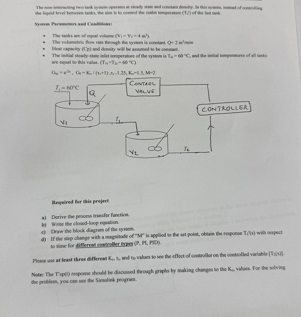
Give step-by-step solution with explanation and final answer:The non-interacting two tank system operates at steady state and constant den:
s at steady state and constant density. In his system, in
the liquid level between tanks, the aim is to control the outlet temperatiire psi hid stead of controlling
System Parameters and Conditions:
+ The tanks are of equal volume (Vy = V3 = 4 m).
«The volumetric flow rate through the system is constant. Q= 2 m/min
«Heat capacity (Cp) and density will be assumed to be constant.
© Theinitial steady-state inlet tem gi
perature of the system is Tin = 60 ° po
Bir nian nal ystem is Tin = 60 °C, and the initial temperatures of ail tanks
Ga =e, Gr=Ku/ (x) 11.25, K=1.5, M=2
7,= 60°C ConteoL
Q NaLvE
l
ne I
ER
le 2) 2
Required for this project
2) Derive the process transfer function.
b) Write the closed-loop equation.
©) Draw the block diagram of the system.
d) Ifthe step change with a magnitude of “Mis applied to the set point, obtain the response T2/(s) with respect
to time for different controller s (P, PI, PID).
Please use at least three different Ke, Ti, and tp values to see the effect of controller on the controlled variable [T2(s)]
Note: The T'sp(t) response should be discussed through graphs by making changes to the Ke, values. For the solving
the problem, you can use the Simulink program.
Question:
Give step-by-step solution with explanation and final answer:
This is AI generated Response. Asked by: Francis Created at: 2025-12-30 04:35:36
Did you like this answer?
👍 0
👎 0
Let's solve the problem step by step as requested:
---
# **(a) Derive the Process Transfer Function**
## **System Description**
- Two non-interacting tanks in series.
- Each tank: \( V_1 = V_2 = 4\, m^3 \)
- Flow rate: \( Q = 2\, m^3/\text{min} \)
- Inlet temperature: \( T_{in} = 60^\circ C \)
- Initial temperature: \( T_1 = T_2 = 60^\circ C \)
- Heat capacity and density are constant.
- Goal: Control outlet temp (\(T_2\)) by adjusting the inlet temp (\(T_{in}\)), using a control valve and controller.
## **Step 1: Write the dynamic equations**
For **Tank 1** (non-interacting, well-mixed):
\[
V_1 \frac{dT_1}{dt} = Q(T_{in} - T_1)
\]
\[
\Rightarrow \frac{dT_1}{dt} + \frac{Q}{V_1}T_1 = \frac{Q}{V_1}T_{in}
\]
For **Tank 2**:
\[
V_2 \frac{dT_2}{dt} = Q(T_1 - T_2)
\]
\[
\Rightarrow \frac{dT_2}{dt} + \frac{Q}{V_2}T_2 = \frac{Q}{V_2}T_1
\]
## **Step 2: Laplace Transform**
Let’s take Laplace transforms (assuming zero initial conditions):
\[
V_1 [sT_1(s)] + Q T_1(s) = Q T_{in}(s)
\]
\[
\Rightarrow (V_1 s + Q)T_1(s) = Q T_{in}(s)
\]
\[
\Rightarrow T_1(s) = \frac{Q}{V_1 s + Q} T_{in}(s)
\]
Similarly, for Tank 2:
\[
(V_2 s + Q) T_2(s) = Q T_1(s)
\]
\[
\Rightarrow T_2(s) = \frac{Q}{V_2 s + Q} T_1(s)
\]
## **Step 3: Overall Transfer Function**
Combine the above:
\[
T_2(s) = \frac{Q}{V_2 s + Q} \cdot \frac{Q}{V_1 s + Q} T_{in}(s)
\]
Given \( V_1 = V_2 = 4 \), \( Q = 2 \):
\[
T_2(s) = \left( \frac{2}{4s + 2} \right)^2 T_{in}(s)
= \left( \frac{1}{2s + 1} \right)^2 T_{in}(s)
\]
So the **process transfer function** is:
\[
\boxed{ G_p(s) = \frac{T_2(s)}{T_{in}(s)} = \frac{1}{(2s+1)^2} }
\]
---
# **(b) Write the Closed-Loop Equation**
Let \( G_c(s) \) be the controller transfer function The block diagram is:
- Controller: \( G_c(s) \)
- Process: \( G_p(s) \)
- Unity feedback.
The closed-loop transfer function is:
\[
T_{cl}(s) = \frac{G_c(s) G_p(s)}{1 + G_c(s) G_p(s)}
\]
Where:
- \( G_p(s) = \frac{1}{(2s+1)^2} \)
- \( G_c(s) \) depends on controller type (P, PI, PID).
---
# **(c) Draw the Block Diagram**
**Block Diagram Structure:**
```
+-----------+ +-----------+ +--------+
Setpoint --->| Controller |--->| Process |--->| Output |
+-----------+ (G_p(s)) +--------+
| ^
+---------------+
```
- Setpoint minus Output feeds the Controller.
- Controller output feeds the Process (plant).
- Process output is the system output (T2).
---
# **(d) Response for Different Controllers**
## **1. Proportional Controller (P)**
\[
G_c(s) = K_c
\]
Closed-loop TF:
\[
T_{cl, P}(s) = \frac{K_c G_p(s)}{1 + K_c G_p(s)}
= \frac{K_c}{(2s+1)^2 + K_c}
\]
## **2. Proportional-Integral Controller (PI)**
\[
G_c(s) = K_c \left( 1 + \frac{1}{\tau_I s} \right)
\]
Closed-loop TF:
\[
T_{cl, PI}(s) = \frac{K_c \left(1 + \frac{1}{\tau_I s}\right) G_p(s)}{1 + K_c \left(1 + \frac{1}{\tau_I s}\right) G_p(s)}
\]
## **3. Proportional-Integral-Derivative Controller (PID)**
\[
G_c(s) = K_c \left( 1 + \frac{1}{\tau_I s} + \tau_D s \right)
\]
Closed-loop TF:
\[
T_{cl, PID}(s) = \frac{K_c \left(1 + \frac{1}{\tau_I s} + \tau_D s\right) G_p(s)}{1 + K_c \left(1 + \frac{1}{\tau_I s} + \tau_D s\right) G_p(s)}
\]
---
# **Response to Step Input**
For a step change of magnitude \( M \):
- Input: \( R(s) = \frac{M}{s} \)
- Output: \( T_2(s) = T_{cl}(s) \cdot R(s) \)
**You can analyze the time response by inverse Laplace or using MATLAB/Simulink.**
---
# **Parameter Values**
Try **at least three different sets** for \( K_c, \tau_I, \tau_D \) to see the effect.
---
# **Summary of Answers**
### **(a) Process Transfer Function**
\[
\boxed{ G_p(s) = \frac{1}{(2s+1)^2} }
\]
### **(b) Closed-Loop Equation**
\[
\boxed{ T_{cl}(s) = \frac{G_c(s) G_p(s)}{1 + G_c(s) G_p(s)} }
\]
### **(c) Block Diagram**
- **Setpoint → Controller → Process → Output**
- **Output is fed back (negative feedback) to compare with setpoint**
### **(d) Response with Different Controllers**
- Use \( T_{cl}(s) \) for each controller type.
- For a step input: \( T_2(s) = T_{cl}(s) \cdot \frac{M}{s} \)
- Plot for at least three sets of controller parameters.
---
## **Tip**
For simulation and plotting, use Simulink/MATLAB as instructed, and change \( K_c, \tau_I, \tau_D \) values to analyze the system's behavior under P, PI, and PID control.
---
**If you need help with the Simulink implementation or specific parameter analysis, let me know!**
📢 Instructions:
Ask anything relatd to above question only.
For new Question goto :
🚀 Submit (-0.25 Credits🪙)
Study Help, Fast Answers
VIPSolutions focuses on clear, step‑by‑step explanations so you can learn quickly. Whether you need an AI‑generated walkthrough or a short hint to get unstuck, each solution is organized for fast reading and easy review later.
Search similar questions, compare approaches, and bookmark the best answers for revision. Our goal is simple: quick, reliable study help that feels natural—not noisy.
 The non-interacting two tank system operates at steady state and constant den:
s at steady state and constant density. In his system, in
the liquid level between tanks, the aim is to control the outlet temperatiire psi hid stead of controlling
System Parameters and Conditions:
+ The tanks are of equal volume (Vy = V3 = 4 m).
«The volumetric flow rate through the system is constant. Q= 2 m/min
«Heat capacity (Cp) and density will be assumed to be constant.
© Theinitial steady-state inlet tem gi
perature of the system is Tin = 60 ° po
Bir nian nal ystem is Tin = 60 °C, and the initial temperatures of ail tanks
Ga =e, Gr=Ku/ (x) 11.25, K=1.5, M=2
7,= 60°C ConteoL
Q NaLvE
l
ne I
ER
le 2) 2
Required for this project
2) Derive the process transfer function.
b) Write the closed-loop equation.
©) Draw the block diagram of the system.
d) Ifthe step change with a magnitude of “Mis applied to the set point, obtain the response T2/(s) with respect
to time for different controller s (P, PI, PID).
Please use at least three different Ke, Ti, and tp values to see the effect of controller on the controlled variable [T2(s)]
Note: The T'sp(t) response should be discussed through graphs by making changes to the Ke, values. For the solving
the problem, you can use the Simulink program.
The non-interacting two tank system operates at steady state and constant den:
s at steady state and constant density. In his system, in
the liquid level between tanks, the aim is to control the outlet temperatiire psi hid stead of controlling
System Parameters and Conditions:
+ The tanks are of equal volume (Vy = V3 = 4 m).
«The volumetric flow rate through the system is constant. Q= 2 m/min
«Heat capacity (Cp) and density will be assumed to be constant.
© Theinitial steady-state inlet tem gi
perature of the system is Tin = 60 ° po
Bir nian nal ystem is Tin = 60 °C, and the initial temperatures of ail tanks
Ga =e, Gr=Ku/ (x) 11.25, K=1.5, M=2
7,= 60°C ConteoL
Q NaLvE
l
ne I
ER
le 2) 2
Required for this project
2) Derive the process transfer function.
b) Write the closed-loop equation.
©) Draw the block diagram of the system.
d) Ifthe step change with a magnitude of “Mis applied to the set point, obtain the response T2/(s) with respect
to time for different controller s (P, PI, PID).
Please use at least three different Ke, Ti, and tp values to see the effect of controller on the controlled variable [T2(s)]
Note: The T'sp(t) response should be discussed through graphs by making changes to the Ke, values. For the solving
the problem, you can use the Simulink program.