Give step-by-step solution with explanation and final answer:Problem: Market Analysis with an Excise Tax
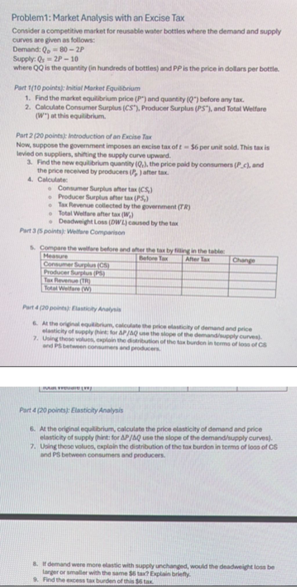
Consider a competitive market for reusable water bottles where the demand and supply
curves e

Question

Give step-by-step solution with explanation and final answer:Problem: Market Analysis with an Excise Tax
Consider a competitive market for reusable water bottles where the demand and supply
curves ee given as follows:
Demand: Qp += 80 ~ 2P
Supply: Qs = 2P = 10
whore QQ is the quantity (in hundreds of bottles) and PP is the price in dollars per bottle.
Part 1(10 points): Initial Market Equilibrium
1. Find the market equilibrium price (P*) and quantity (Q*) before any tax.
2. Calculate Consumer Surplus (CS*), Producer Surplus (PS*), and Total Welfare
(W*) at this equilibrium.
Part 2 (20 points): Introduction of an Excise Tax
Now, suppose the government imposes an excise tax of t = $6 per unit sold. This tax is
loviod on suppliers, shifting the supply curve upward.
3 Find the new equilibrium quantity (Q,), the price pad by consumers (P_c), and
the price received by producers (F), ) after tax.
4. Coleulate:
° Consumer Surplus after tax (CS)
o Producer Surplus after tax (PS,)
° Tax Revenue collected by the government (TR)
© Total Welfare after tax (W,)
© Deadweight Loss (DWL) caused by the tax
Part 3 (5 points): Weltare Comparison
Compare the welfare before snd aft

VIPSolutions · Accepted Answer

Let's solve the problem step-by-step, as requested.

---

# **Problem 1: Market Analysis with an Excise Tax**

### **Given:**

- **Demand:** $ Q_D = 80 - 2P $
- **Supply:** $ Q_S = 2P - 10 $
- $ Q $ is in hundreds of bottles, $ P $ is in dollars per bottle.

---

## **Part 1: Initial Market Equilibrium**

### **1. Find Equilibrium Price ($ P^* $) and Quantity ($ Q^* $)**

Set $ Q_D = Q_S $:

$$
80 - 2P = 2P - 10
$$
$$
80 + 10 = 2P + 2P
$$
$$
90 = 4P
$$
$$
P^* = 22.5
$$

Plug $ P^* $ into either curve to get $ Q^* $:

$$
Q^* = 80 - 2(22.5) = 80 - 45 = 35
$$

(So, **$ Q^* = 35 $ hundreds = 350 bottles**)

---

### **2. Calculate Consumer Surplus (CS), Producer Surplus (PS), and Total Welfare (W)**

#### **Find intercepts:**

- **Demand:** $ Q_D =  \implies 80 - 2P =  \implies P = 40 $
- **Supply:** $ Q_S =  \implies 2P - 10 =  \implies P = 5 $

#### **Formulas:**

- **CS:** Area above $ P^* $ and below demand curve
$$
CS = \frac{1}{2} (Q^*) (P_{max} - P^*)
$$
- **PS:** Area below $ P^* $ and above supply curve
$$
PS = \frac{1}{2} (Q^*) (P^* - P_{min})
$$
- **Total Welfare:** $ W = CS + PS $

#### **Calculations:**

- **CS:**
$$
CS = \frac{1}{2} \times 35 \times (40 - 22.5) = \frac{1}{2} \times 35 \times 17.5 = 306.25
$$

- **PS:**
$$
PS = \frac{1}{2} \times 35 \times (22.5 - 5) = \frac{1}{2} \times 35 \times 17.5 = 306.25
$$

- **Total Welfare:**
$$
W = 306.25 + 306.25 = 612.5
$$

---

## **Part 2: Introduction of an Excise Tax ($ t = \$6 $)**

The new supply curve shifts up by $6:  
$$
Q_S = 2(P - 6) - 10 = 2P - 12 - 10 = 2P - 22
$$

Set new supply equal to demand for equilibrium:

$$
80 - 2P = 2P - 22
$$
$$
80 + 22 = 2P + 2P
$$
$$
102 = 4P \implies P_c = 25.5
$$

- **Price received by producers:** $ P_p = P_c - 6 = 25.5 - 6 = 19.5 $
- **Quantity after tax:** $ Q_t = 80 - 2 \times 25.5 = 80 - 51 = 29 $

---

### **4. Calculate After-Tax Values**

- **Consumer Surplus after tax ($ CS_2 $):**
$$
CS_2 = \frac{1}{2} \times 29 \times (40 - 25.5) = \frac{1}{2} \times 29 \times 14.5 = 210.25
$$

- **Producer Surplus after tax ($ PS_2 $):**
$$
PS_2 = \frac{1}{2} \times 29 \times (19.5 - 5) = \frac{1}{2} \times 29 \times 14.5 = 210.25
$$

- **Tax Revenue ($ TR $):**
$$
TR = t \times Q_t = 6 \times 29 = 174
$$

- **Total Welfare after tax ($ W_2 $):**
$$
W_2 = CS_2 + PS_2 + TR = 210.25 + 210.25 + 174 = 594.5
$$

- **Deadweight Loss ($ DWL $):**
$$
DWL = W - W_2 = 612.5 - 594.5 = 18
$$

---

## **Part 3: Welfare Comparison Table**

| Measure           | Before Tax | After Tax | Change   |
|-------------------|------------|-----------|----------|
| Consumer Surplus  | 306.25     | 210.25    | -96      |
| Producer Surplus  | 306.25     | 210.25    | -96      |
| Tax Revenue       |           | 174       | +174     |
| Total Welfare     | 612.5      | 594.5     | -18      |

---

## **Part 4: Elasticity Analysis**

### **6. Price Elasticity at Equilibrium**

Recall:
- $ Q^* = 35 $, $ P^* = 22.5 $
- Demand curve slope = $-2$; Supply curve slope = $2$

#### **Elasticity of Demand:**

$$
E_d = \frac{dQ}{dP} \cdot \frac{P^*}{Q^*} = (-2) \cdot \frac{22.5}{35} = -1.29
$$

#### **Elasticity of Supply:**

$$
E_s = \frac{dQ}{dP} \cdot \frac{P^*}{Q^*} = 2 \cdot \frac{22.5}{35} = 1.29
$$

---

### **7. Tax Burden Distribution**

- Both elasticities are equal in magnitude.
- Thus, the tax burden (loss in CS and PS) is **shared equally** between consumers and producers.

---

### **8. Effect of More Elastic Demand**

- **If demand is more elastic:** Deadweight loss **increases** because the reduction in quantity traded is larger for a given tax.

---

### **9. Excess Tax Burden (DWL)**

$$
\boxed{DWL = 18}
$$

---

## **Summary Table**

| Measure           | Before Tax | After Tax | Change   |
|-------------------|------------|-----------|----------|
| Consumer Surplus  | 306.25     | 210.25    | -96      |
| Producer Surplus  | 306.25     | 210.25    | -96      |
| Tax Revenue       |           | 174       | +174     |
| Total Welfare     | 612.5      | 594.5     | -18      |
| Deadweight Loss   |           | 18        | +18      |

---

## **Final Answers**
- **Equilibrium price and quantity (before tax):** $ P^* = \$22.5 $, $ Q^* = 35 $ (hundreds)
- **Equilibrium after tax:** $ Q_t = 29 $, $ P_c = \$25.5 $, $ P_p = \$19.5 $
- **Consumer Surplus before/after:** 306.25 / 210.25
- **Producer Surplus before/after:** 306.25 / 210.25
- **Tax Revenue:** 174
- **Total Welfare before/after:** 612.5 / 594.5
- **Deadweight Loss:** 18

Let me know if you need the graph or any particular step explained in more detail!

✨ VIPSolutions

Question:

Final Answer:

📢 Instructions:

Study Help, Fast Answers

✨ VIPSolutions

Question:

Final Answer:

📢 Instructions:

Related Answers

Study Help, Fast Answers