Give step-by-step solution with explanation and final answer:= Elles flere oi mE lea ea pd mss RE
mee
= El ee i ie ey il
(a) Consider the followmg autoregressive proc amen 0
Seale se Be EE
| uae oan) EE ie
oEdEGR no . .
he pre fom pee ees ps prs
el nh ie dg Seren
Semis op a
s Hkmimoema ERY eh ch Ln
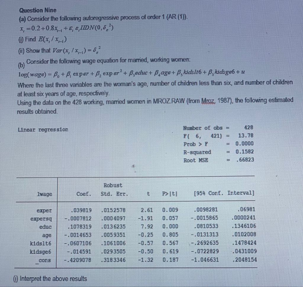
. Using he data on tre 428 working, married women in MROZRAW (from Mroz, 1987), the following estimated
| reecbbeed. —
Upear regress. | Mumberofobs= 428
Ca : E( 6 421) = 13.78
Le ! | Prob > F = 0.0000
0 | R-squared = 0.1582
Sa i Root MSE = .66823
i Al
—- Robust
| dwage | roer. | Sta, Err, Lt Pit [95% Conf. Interval] |
emer | 03m 0152578 2.61 0.009 .0098281 06981
epersq | -.0007812 0004097 -1.91 0.057 -.0015865 .0000241
| educ | 1078319 0136235 7.92 0.000 .0810533 .1346106
age | -.D00I4653 .0059351 0.25 (0.805 -.0131313 0102008
Kdsit6 | -.0607106 1061006 -0.57 0.567 -.2692635 .1478424 LL
kidsgef | -.014591 0293505 0.50 0.619 -.0722829 .D431009 hy
cons | -.4709078 3183346 1.32 0.187 -1.046631 .2046154 En
ee - = GE
ee: =
Gi Ee ER ; iE en EE EEA
Question:
Give step-by-step solution with explanation and final answer:= Elles flere oi mE lea ea pd mss RE
mee
= El ee i ie ey il
(a) Consider the followmg autoregressive proc amen 0
Seale se Be EE
| uae oan) EE ie
oEdEGR no . .
he pre fom pee ees ps prs
el nh ie dg Seren
Semis op a
s Hkmimoema ERY eh ch Ln
. Using he data on tre 428 working, married women in MROZRAW (from Mroz, 1987), the following estimated
| reecbbeed. —
Upear regress. | Mumberofobs= 428
Ca : E( 6 421) = 13.78
Le ! | Prob > F = 0.0000
0 | R-squared = 0.1582
Sa i Root MSE = .66823
i Al
—- Robust
| dwage | roer. | Sta, Err, Lt Pit [95% Conf. Interval] |
emer | 03m 0152578 2.61 0.009 .0098281 06981
epersq | -.0007812 0004097 -1.91 0.057 -.0015865 .0000241
| educ | 1078319 0136235 7.92 0.000 .0810533 .1346106
age | -.D00I4653 .0059351 0.25 (0.805 -.0131313 0102008
Kdsit6 | -.0607106 1061006 -0.57 0.567 -.2692635 .1478424 LL
kidsgef | -.014591 0293505 0.50 0.619 -.0722829 .D431009 hy
cons | -.4709078 3183346 1.32 0.187 -1.046631 .2046154 En
ee - = GE
ee: =
Gi Ee ER ; iE en EE EEA
This is AI generated Response.
Asked by: Sahzadi
Created at: 2026-03-07 21:41:05
Final Answer:
RenderedRaw Text
Did you like this answer?
Let's break down and solve the problem step by step:
---
# **(a) Autoregressive Process AR(1)**
Given:
\[
x_t = .2 + .8x_{t-1} + \epsilon_t, \quad \epsilon_t \sim IIDN(, \sigma^2)
\]
---
## **(i) Find \( E(x_t | x_{t-1}) \):**
The conditional expectation is:
\[
E(x_t | x_{t-1}) = E[.2 + .8x_{t-1} + \epsilon_t \mid x_{t-1}]
\]
Since \( \epsilon_t \) is independent of \( x_{t-1} \) and has mean zero:
\[
E(x_t | x_{t-1}) = .2 + .8x_{t-1} + E(\epsilon_t) = .2 + .8x_{t-1}
\]
---
## **(ii) Show that \( Var(x_t | x_{t-1}) = \sigma^2 \):**
Conditional variance:
\[
Var(x_t | x_{t-1}) = Var(.2 + .8x_{t-1} + \epsilon_t \mid x_{t-1})
\]
\(.2 + .8x_{t-1}\) is just a constant given \(x_{t-1}\), so the variance is just the variance of \( \epsilon_t \):
\[
Var(x_t | x_{t-1}) = Var(\epsilon_t) = \sigma^2
\]
---
# **(b) Wage Equation for Married, Working Women**
Model:
\[
\log(wage) = \beta_ + \beta_1 \text{exper} + \beta_2 \text{exper}^2 + \beta_3 \text{educ} + \beta_4 \text{age} + \beta_5 \text{kidslt6} + \beta_6 \text{kidsge6} + u
\]
Regression summary (key coefficients):
| Variable | Coef. | Std. Err. | t | P>|t| | 95% Conf. Interval |
|-----------|------------|-----------|-------|------|-----------------------------|
| exper | .039819 | .015258 | 2.61 | .009| [.009281, .06981] |
| expersq | -.0007812 | .0004097 | -1.91 | .057| [-.001586, .000241] |
| educ | .1078319 | .0136235 | 7.92 | .000| [.081053, .1346016] |
| age | -.001463 | .0059351 | -.25 | .805| [-.013313, .010208] |
| kidslt6 | -.0607106 | .1061006 | -.57 | .567| [-.269263, .147824] |
| kidsge6 | -.014591 | .0293505 | -.50 | .619| [-.072289, .043109] |
| _cons | -.4290078 | .3183346 | -1.32 | .187| [-1.046631, .2041854] |
---
## **(c) Interpret the Results**
### **Statistical Significance (P-values):**
- **Experience (\(exper\))**: Significant positive effect (\(p = .009 < .05\)). Each year of experience increases log(wage) by about .04, holding other variables constant.
- **Experience squared (\(expersq\))**: Marginally significant (\(p = .057\)), negative coefficient suggests diminishing returns to experience.
- **Education (\(educ\))**: Highly significant (\(p = .000\)), positive effect. Each year of education increases log(wage) by about .108.
- **Age**: Not significant (\(p = .805\)), effect is close to zero.
- **Children under 6 (\(kidslt6\))**: Not significant (\(p = .567\)), small negative effect.
- **Children 6 or older (\(kidsge6\))**: Not significant (\(p = .619\)), very small negative effect.
- **Constant**: Not significant (\(p = .187\)).
### **Model Fit:**
- \(R^2 = .1582\): The model explains about 15.8% of the variation in log(wage).
- \(F(6, 421) = 13.78\), \(p < .001\): Model is jointly significant.
### **Economic Interpretation:**
- **Experience and Education**: Both are important for higher wages (statistically significant), though the effect of experience diminishes at higher levels.
- **Age and Children**: No significant effect on wages found for age or for having children, whether under 6 or older.
---
## **Summary Table**
| Variable | Effect on log(wage) | Significance | Interpretation |
|------------|--------------------|--------------|-----------------------------------------------------|
| exper | Positive | Significant | Experience increases wages; effect diminishes at higher experience (see expersq). |
| educ | Positive | Significant | More education increases wages. |
| age | Near zero | Not significant | No strong evidence age matters after controlling for other factors. |
| kidslt6 | Slight negative | Not significant | Having young children does not significantly affect wages. |
| kidsge6 | Slight negative | Not significant | Having older children does not significantly affect wages. |
---
## **Final Answers**
### **(a)**
1. \( E(x_t | x_{t-1}) = .2 + .8x_{t-1} \)
2. \( Var(x_t | x_{t-1}) = \sigma^2 \)
### **(b)**
- Experience and education significantly increase wages for married, working women.
- Age and having children (either under or over 6) do not significantly affect wages.
- The model explains a moderate share (15.8%) of the variation in wages.
---
**If you need further breakdown of the math or more detail in interpretation, just ask!**
VIPSolutions focuses on clear, step‑by‑step explanations so you can learn quickly. Whether you need an AI‑generated walkthrough or a short hint to get unstuck, each solution is organized for fast reading and easy review later.
Search similar questions, compare approaches, and bookmark the best answers for revision. Our goal is simple: quick, reliable study help that feels natural—not noisy.
 = Elles flere oi mE lea ea pd mss RE
mee
= El ee i ie ey il
(a) Consider the followmg autoregressive proc amen 0
Seale se Be EE
| uae oan) EE ie
oEdEGR no . .
he pre fom pee ees ps prs
el nh ie dg Seren
Semis op a
s Hkmimoema ERY eh ch Ln
. Using he data on tre 428 working, married women in MROZRAW (from Mroz, 1987), the following estimated
| reecbbeed. —
Upear regress. | Mumberofobs= 428
Ca : E( 6 421) = 13.78
Le ! | Prob > F = 0.0000
0 | R-squared = 0.1582
Sa i Root MSE = .66823
i Al
—- Robust
| dwage | roer. | Sta, Err, Lt Pit [95% Conf. Interval] |
emer | 03m 0152578 2.61 0.009 .0098281 06981
epersq | -.0007812 0004097 -1.91 0.057 -.0015865 .0000241
| educ | 1078319 0136235 7.92 0.000 .0810533 .1346106
age | -.D00I4653 .0059351 0.25 (0.805 -.0131313 0102008
Kdsit6 | -.0607106 1061006 -0.57 0.567 -.2692635 .1478424 LL
kidsgef | -.014591 0293505 0.50 0.619 -.0722829 .D431009 hy
cons | -.4709078 3183346 1.32 0.187 -1.046631 .2046154 En
ee - = GE
ee: =
Gi Ee ER ; iE en EE EEA
= Elles flere oi mE lea ea pd mss RE
mee
= El ee i ie ey il
(a) Consider the followmg autoregressive proc amen 0
Seale se Be EE
| uae oan) EE ie
oEdEGR no . .
he pre fom pee ees ps prs
el nh ie dg Seren
Semis op a
s Hkmimoema ERY eh ch Ln
. Using he data on tre 428 working, married women in MROZRAW (from Mroz, 1987), the following estimated
| reecbbeed. —
Upear regress. | Mumberofobs= 428
Ca : E( 6 421) = 13.78
Le ! | Prob > F = 0.0000
0 | R-squared = 0.1582
Sa i Root MSE = .66823
i Al
—- Robust
| dwage | roer. | Sta, Err, Lt Pit [95% Conf. Interval] |
emer | 03m 0152578 2.61 0.009 .0098281 06981
epersq | -.0007812 0004097 -1.91 0.057 -.0015865 .0000241
| educ | 1078319 0136235 7.92 0.000 .0810533 .1346106
age | -.D00I4653 .0059351 0.25 (0.805 -.0131313 0102008
Kdsit6 | -.0607106 1061006 -0.57 0.567 -.2692635 .1478424 LL
kidsgef | -.014591 0293505 0.50 0.619 -.0722829 .D431009 hy
cons | -.4709078 3183346 1.32 0.187 -1.046631 .2046154 En
ee - = GE
ee: =
Gi Ee ER ; iE en EE EEA