Give step-by-step solution with explanation and final answer:Justice Computers, a major PC manufacturer in Canada, currently has a plant in Toronto. The Toronto plant has a capacity of 1 million units a year. The firm divides Canada into five markets: Atlantic, Central, Prairie, Pacific and Territories. Each PC sells for $1,800. The firm wants to build a couple of plants, each plant with a capacity of 1.6 million units per year, to accommodate the growth. Potential sites being considered are Halifax, Winnipeg and Vancouver. Annual fixed costs, production and shipping costs per unit, and the expected regional demand are shown in the following Table. | eee | $/Unit IE DVO 0 FOO FO PO == Atlantic Central | Prairies | Pacific | Territories | Cost (Million § | Toronto | 180 | iso [ 175s [19s | 21s [100 | | Mafox | 170 | 190 | 180 | 210 | 235 [iso | | winnipeg | 185 | iso [ 18s | 200 [ 20s [75 | Demand kAMMNN NN units/year, 600 400 700 300 1) If Blue Computers sets an objective of minimizing the total cost, where should it build the new plant? How should the network be structured? To solve the problem a) Formulate the problem with mathematical models (MIP) b) Solve it with the Excel solver. 2) If each market has single source policy, i.e., only one manufacturer can supply PC to each market, what is your new model and solution? ¢) Formulate the problem with mathematical models (MIP) d) Solve it with the Excel solver.
Question:
Give step-by-step solution with explanation and final answer: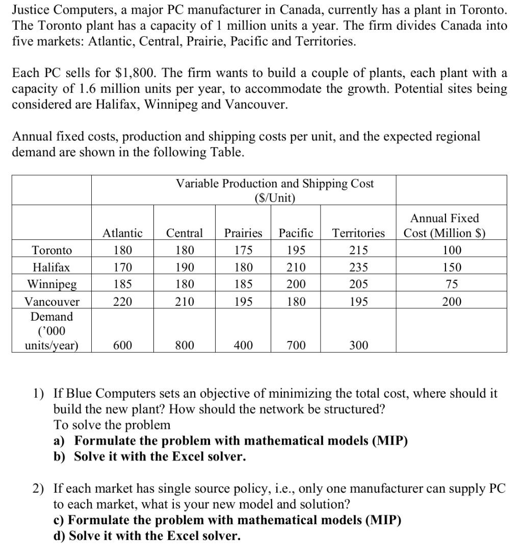 Justice Computers, a major PC manufacturer in Canada, currently has a plant in Toronto.
The Toronto plant has a capacity of 1 million units a year. The firm divides Canada into
five markets: Atlantic, Central, Prairie, Pacific and Territories.
Each PC sells for $1,800. The firm wants to build a couple of plants, each plant with a
capacity of 1.6 million units per year, to accommodate the growth. Potential sites being
considered are Halifax, Winnipeg and Vancouver.
Annual fixed costs, production and shipping costs per unit, and the expected regional
demand are shown in the following Table.
| eee |
$/Unit
IE DVO 0 FOO FO PO ==
Atlantic Central | Prairies | Pacific | Territories | Cost (Million §
| Toronto | 180 | iso [ 175s [19s | 21s [100 |
| Mafox | 170 | 190 | 180 | 210 | 235 [iso |
| winnipeg | 185 | iso [ 18s | 200 [ 20s [75 |
Demand
kAMMNN NN
units/year, 600 400 700 300
1) If Blue Computers sets an objective of minimizing the total cost, where should it
build the new plant? How should the network be structured?
To solve the problem
a) Formulate the problem with mathematical models (MIP)
b) Solve it with the Excel solver.
2) If each market has single source policy, i.e., only one manufacturer can supply PC
to each market, what is your new model and solution?
¢) Formulate the problem with mathematical models (MIP)
d) Solve it with the Excel solver.
Justice Computers, a major PC manufacturer in Canada, currently has a plant in Toronto.
The Toronto plant has a capacity of 1 million units a year. The firm divides Canada into
five markets: Atlantic, Central, Prairie, Pacific and Territories.
Each PC sells for $1,800. The firm wants to build a couple of plants, each plant with a
capacity of 1.6 million units per year, to accommodate the growth. Potential sites being
considered are Halifax, Winnipeg and Vancouver.
Annual fixed costs, production and shipping costs per unit, and the expected regional
demand are shown in the following Table.
| eee |
$/Unit
IE DVO 0 FOO FO PO ==
Atlantic Central | Prairies | Pacific | Territories | Cost (Million §
| Toronto | 180 | iso [ 175s [19s | 21s [100 |
| Mafox | 170 | 190 | 180 | 210 | 235 [iso |
| winnipeg | 185 | iso [ 18s | 200 [ 20s [75 |
Demand
kAMMNN NN
units/year, 600 400 700 300
1) If Blue Computers sets an objective of minimizing the total cost, where should it
build the new plant? How should the network be structured?
To solve the problem
a) Formulate the problem with mathematical models (MIP)
b) Solve it with the Excel solver.
2) If each market has single source policy, i.e., only one manufacturer can supply PC
to each market, what is your new model and solution?
¢) Formulate the problem with mathematical models (MIP)
d) Solve it with the Excel solver.
Asked by: gvr
Created at: 2025-07-25 15:13:14
Final Answer:
📢 Instructions:
- Ask anything relatd to above question only.
- For new Question goto :