Question:

urgent!!! please answer the full question and provide valid excel screenshot. i will upvote. b . Now conduct a sensitivity analysis to determine the sensitivity of NPV to changes in the sales price, variable costs per unit, and number of units sold. Set these variables' values at 1 0 % and 2 0 % above and below their base - case values. Include a graph in your analysis. For example, the base case 1 st Year Unit Sales in Cell B 1 0 0 should be the number 1 , 0 0 0 and NOT have the formula = D 3 1 in 1 0 % Excel will calculate the wrong answer. Unfortunately, Excel won't tell you that there is a problem, so you'll just get the wrong values for the data table! - won't tell you that there is a problem, so you'll just get the Excel will calculate the wrong answer. Unfortunately, Exce won't tell you that there is a problem, so you'll just get the wrong values for the data table! - 1 0 % 0 % 1 0 % 2 0 % Range c . 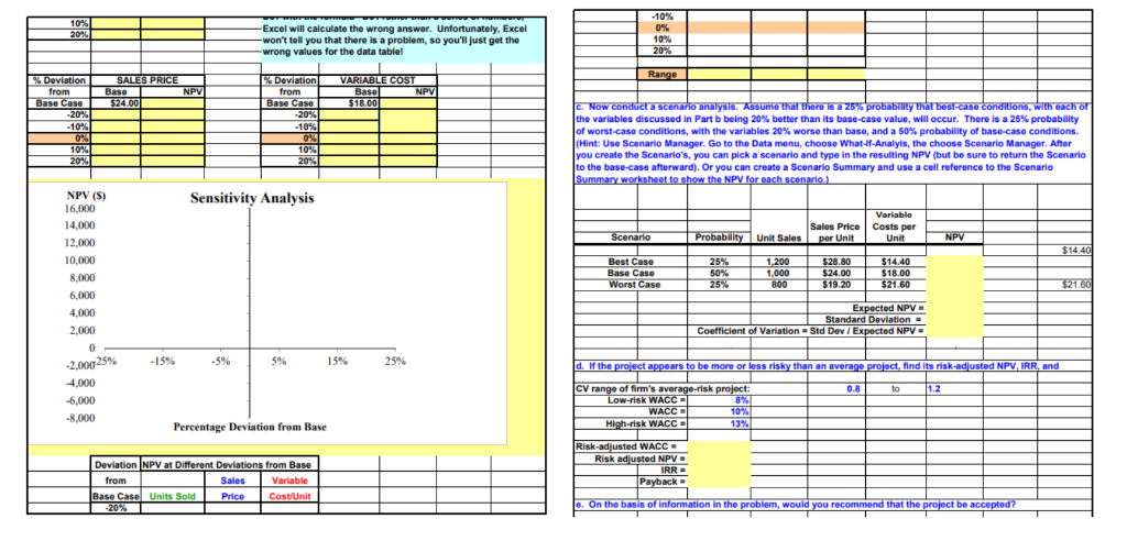Now conduct a scenario analysis. Assume that there is a 2 5 % probability that best - case conditions, with each of the variables discussed in Part b being 2 0 % better than its base - case value, will occur. There is a 2 5 % probability of worst - case conditions, with the variables 2 0 % worse than base, and a 5 0 % probability of base - case conditions. ( Hint: Use Scenario Manager. Go to the Data menu, choose What - If - Analyis, the choose Scenario Manager. After you create the Scenario's, you can pick a scenario and type in the resulting NPV ( but be sure to return the Scenario to the base - case afterward ) . Or you can create a Scenario Summary and use a cell reference to the Scenario Summary worksheet to show the NPV for each scenario. ) Unit Sales Sales Price per Unit Variable Costs per Unit Scenario Probability NPV $ 1 4 . 4 0 Best Case 2 5 % 1 , 2 0 0 $ 2 8 . 8 0 $ 1 4 . 4 0 Base Case 5 0 % 1 , 0 0 0 $ 2 4 . 0 0 $ 1 8 . 0 0 Worst Case 2 5 % 8 0 0 $ 1 9 . 2 0 $ 2 1 . 6 0 $ 2 1 . 6 0 Expected NPV = Standard Deviation = Coefficient of Variation = Std Dev / Expected NPV = d . If the project appears to be more or less risky than an average project, find its risk - adjusted NPV , IRR, and CV range of firm's average - risk project: 0 . 8 to Low - risk WACC = 8 % WACC = 1 0 % High - risk WACC = 1 3 % Risk - adjusted WACC = Risk adjusted NPV = IRR = Payback = e . On the basis of information in the problem, would you recommend that the project be accepted? Scenario Summary Current Values: Base Case Best Case Worst Case Changing Cells: $D$ 2 7 Base Case Base Case Best Case Worst Case $D$ 2 8 5 0 % 5 0 % 2 5 % 2 5 % $D$ 3 1 1 , 0 0 0 1 , 0 0 0 1 , 2 0 0 8 0 0 $D$ 3 2 $ 2 4 . 0 0 $ 2 4 . 0 0 $ 2 8 . 8 0 $ 1 9 . 2 0 $D$ 3 3 $ 1 8 . 0 0 $ 1 8 . 0 0 $ 1 4 . 4 0 $ 2 1 . 6 0 Result Cells: $G$ 3 1 $ 3 , 8 2 0 $ 3 , 8 2 0 $ 3 1 , 4 2 1 - $ 1 5 , 5 1 8 $G$ 3 2 2 2 . 2 % 2 2 . 2 % 9 1 . 5 % #NUM! $G$ 3 3 2 . 8 3 2 . 8 3 1 . 0 6 4 . 0 0 Notes: Current Values column represents values of changing cells at time Scenario Summary Report was created. Changing cells for each scenario are highlighted in gray.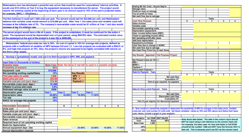a ronnie rl BR or ————— wad com 10 millon Year 81 by ie equipment necessory fo manufacture he server The project would [Emr recur net working capa ot he begin of sach yea in a amt acai 1o 10% of th you rected sie Te i ms — S——— ——— 1 S— — [Th im Baove cout so 000i par year Th savers would el To 534 08 por un 3nd Webasto EE —— — eve ot ai cots wld amu 41000 a ri. Ar Tow 1 sn prc and vu count | [EPI {| & [+ T+ [3 TT th nation rat * omeaabl cons milion Year 1 and io rr — i futon tc 4. To company wed be $1 milion 1 Ve PI —— — - Err er — SE SE ES ES E— —— UC [Th srver rej would ave 3 Wo of year Ws Braet nderavan, Bs Cornus Tor ovr © fom mee ror Te scat wou be Gaeacitd over Sar brio. ing WARS res. Th simaed maton | ischemia ———— | I i EB ys J — Webmasters Tara is sae x ae a 5. con of Copa 3 10% or svar dak raecs, doioed 3 rr — orojects wth a cosficent of variation f NV between 0. and 1.2. Lows projects are ovaated with a WACC o | [Ca fo aoe i change OWE | % and hgh ck projects 133%. Alco th projects returner expected io be Highly corlted wth reume on EE or ee ———— ns i i BS nm J TT ————— Te ee ms ss ms sn ss ——— — Tr —— — ———— ——— C — — = Eo — i — LC e—— I ms mu m— 712 C= — EE — — Cy Ty Crm — 1 — 2 —— — ee ry a —— CC — —— — —— Crea or 1 — Se [J SS SE — yr Fr — 1 ———— — —— J) — ——— — ——— —— —— — Er To I 1 — — ——— LL — ——— TT ——— a 1 SE — 2 So —— ( S—— —— T TTT Er w—— Tf 1 mn mm J Se eS ET ——— | —— ——— —— i i SS ss — — — CE — — J i Js Ss SE — — S————— CE — —— a [eee pees perms asp Coste er senor ed St te aie ven ot 7. nt 37s ho bn [Varibl costs per unt (ct dope] || Jom ws hae» papi Cre rye = —— berm —— LL — 1 — LT ove wr Sas | (Fr —— Not out dase Tecate come pu shots = om —— No oe out ng + a re Cv oO (CEO — Fo emmpe he bse cm i You Unk Bee Con 108 ET Ee = — eT ems 10 i ro rE I —— ate To cas ohn O31 1 nc pt —a=7 1 1 F—F—7—7—] [—=] Exar wit cucute ne wrong snower Urlorumly Excel — ———— — = 108 you that thers is 3 problem, 50 youl just get the. INE TC SN EN ES — I a a Ee es es Es Ee Ee Be sp Es Es Fests i] ES mr 11 J ee ee es ms emt ses pe ss — — Fl] [oes comme ro oy mr se oor oc. Tose vst ET ER — | [of worst-case conditions, with the variables 20% worse than base, and a 0% probability of base-case conditions. = = [an ve Sra an: Get ma ros Wht svat i ns Serato lo = — [es WV ote sone te EE FE — — — beers ne Sensitivity Analysis (7 TT 7 | mm ms ———— pres ——— ——— fe Ee et em — Ee ee ms Ry ms frees Foe Tow | mw | eo ee — on m1 — on es Es es Es — hes EE = — em E— — — 2.000 [TT Coefficient of Variation = Std Dev / Expected NPV = JR E— BH Es a ss Rs I me Sr ET Es —— —— dot E a es ms me es A sess prey Ee Es Es ho e+ Percentage Deiton om He ee —————— ee ee BE Ee Es Es [Risk-adjusted WACC = [ES ES SS — | [empevemsemesmmee] | | [| [| eeeser — tf 5 Ee —— — I E— a 7 E— —— — — Hi ——— — SS C= eee Iu Fe ES I — RY s—— t—(————— 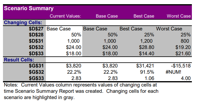Scenario Summary Current Values: Base Case BestCase Worst Case Changing Cells: $D$27 Base Case Base Case Best Case Worst Case $D$28 50% 50% 25% 25% $D$31 1,000 1,000 1,200 800 $D$32 $24.00 $24.00 $28.80 $19.20 $D$33 $18.00 $18.00 $14.40 $21.60 Result Cells: $G$31 $3,820 $3,820 $31,421 -$15,518 $G$32 22.2% 22.2% 91.5% #NUM! $G$33 2.83 2.83 1.06 4.00 Notes: Curent Values column represents values of changing cells at time Scenario Summary Report was created. Changing cells for each scenario are highlighted in gray.